Analysis of the characteristics of a semi with DP shows that due to the wave + noise filter in the DP controller, a sudden disturbance is not effectively countered by the DP system. A third effect may be that of extreme wave driving (i.e., extreme for the wave height), that is, the slowly varying force caused by nonlinear forcing mechanism in irregular seas. The response of the DP system to the wave disturbance will be less immediate than that of mooring system.
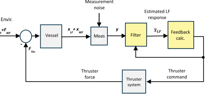
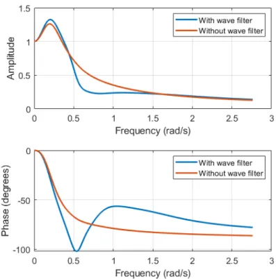
The purpose of the filter is to remove the high frequency (WF) component of the wave from the measured position to leave the low frequency (LF) motion component.
Slamming load
The height h of the slamming area is taken as the most likely highest wave amplitude for three hours. It is pointed out that the calculation of the slam load is rather crude and rests on a number of assumptions. Changing the wave parameters and the duration of the time period in question will not produce drastic changes.
For a square column and when the wave hits one side perpendicularly, it must be assumed that the peak load will be greater and the duration of the load will be shorter.
Wave frequency viscous load
If the wave hits the front of the semi in such a way that the slamming conditions are fulfilled for each of the two front columns, the impulse load will be doubled, and we get:. In both cases, the force-time-duration magnitude of the impulse may not deviate substantially from the estimate for the circular cross-section above. Here u(z) is the depth-dependent speed of water normal to the column's surface, 𝜋𝜋 the water density and D the diameter of the column.
Now assuming a sinusoidal wave with this amplitude, the second integral in (12) is evaluated from the bottom of the column at 9.5 m below the SWL (d in Eq.
Wave-drift load
For a wave of amplitude 6.7 m, the viscous force corresponding to a wave trough is -125 kN on a corner column. The cause of the damage was estimated to be the great force in the middle of the picture. It is characteristic of the wave motion load that does not change sign, although the wave oscillates around the SWL.
Wave driving coefficients are calculated by methods based on potential theory, i.e. the assumption of inviscid fluid flow.

Model
The thruster response (to the thruster command) will, for a real system, be non-linear due to the quadratic hydrodynamic torque drag. However, the thruster's response will also depend on the function of the servo system, which is manufacturer dependent. This frequency will be close to the peak frequency of the wave spectrum, and the width of the spectrum is expected to be comparable to that of the wave spectrum as long as the horizontal WF motion is taken into account.
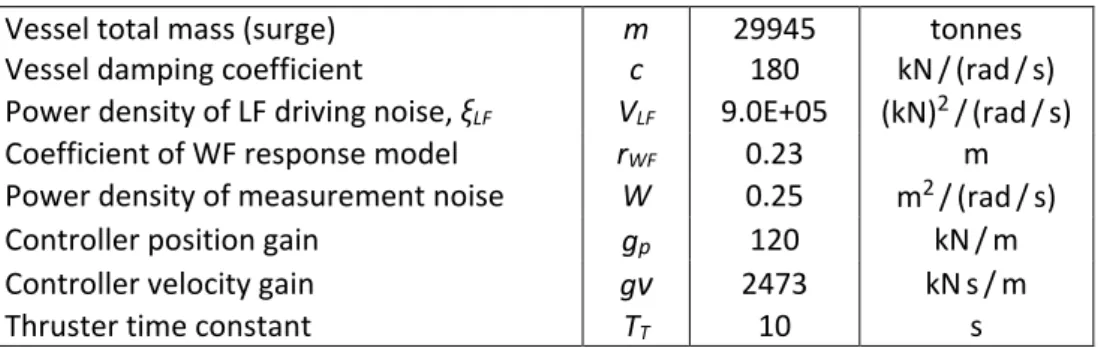
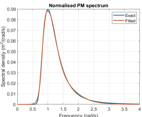
The coefficient rWF can be considered as an average RAO over the width of the wave spectrum (It is noted that the purpose of the WF model is to have a basis for the construction of the wave filter used by the controller (Figure 2-1) and not a high-precision model for the WF reaction). A model order of six was found to give an excellent representation of the P-M spectrum, as demonstrated by Figure 5-1. The WF state space model is made to represent a normalized P-M spectrum, that is, the spectrum corresponding to Hs = 1.0 and Tp = 1.0.
Its task is to make an estimate of the LF state, xLF = [xLF, vLF]T given the measurement, y. In addition to the coefficients of the matrices in the state space model, the (constant) power densities of the process noises (ξLF and ξWF) and the measurement noise (w) must be known. The details of the estimator are not given here, but can be found in [11] or elsewhere in the rich literature on the subject.
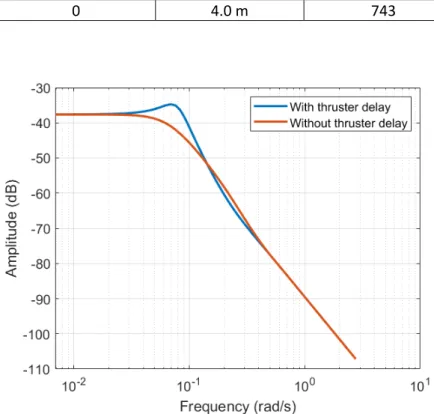
Once the estimate (𝒙𝒙�𝑳𝑳𝑳𝑳) of the LF mode is obtained, the feedback command to the thrusters is expressed as. The speed of the response is determined by the time constant TT, see Figure 5-2, which shows the thruster's response to a unit step in the commanded thrust.
Example
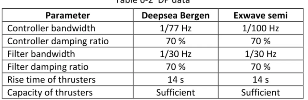
Model data
After a time equal to the time constant, the thrust reached 63% of the final value.
Filter characteristics
Response of dynamically positioned vessel
- Response with and without thruster delay
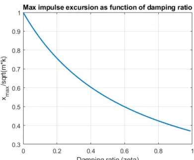
- Analysis of impulse response
- Importance of the initial state
The maximum excursion is 15.2 m, which is more than twice that of the delay-free mass-damper-spring model in Section 3.1, which is shown in blue and labeled “Ideal” in the text box. The reasons for the difference are, as mentioned, the delays in the state estimator (filter) and the thruster's response. The former can be seen from the yellow line in the figure, which shows the estimated position.
According to the figure, the load I1 gives an initial velocity of almost 0.9 m/s in both the ideal (=delay-free) case and the true (or actual) case. In the actual case, the damping is achieved based on the estimated speed and needs some time to take full effect. The maximum position deviation is now 11.4 m, which is still significantly higher than the maximum of 7 m in the ideal case.
This load causes a deflection of up to 2.4 m when the filter and thruster decelerations are taken into account (versus 1.2 m ideally). In the case where the pulse length is 60 seconds, the maximum deflection is almost as low as the maximum in the case of a delay-free control system. In the previous section, an excursion peak of 2.4 m was found for the slamming event described in section 3.1 when the delays in the DP system were included in the calculation.
In the calculation of the load, it was assumed that the wave that caused the shock load forms a vertical wall just before impacting the columns of the semi-submersible vessel. Also, the velocity at the moment of impact can be positive and increase due to the load.
SIMO model
The DP controller in SIMO uses PID control based on state estimates from a quasi-Kalman observer. The intention was to make the DP system in SIMO look like the DP system in the simplified model in Chapter 5. The coefficients of the filter are also functions of the chosen bandwidth and attenuation ratio.
Consequently, the filter characteristic is not based on assumptions of the power spectral density of process noise and measurement noise, as was the basis for the Kalman-Bucy filter used above. The adaptive wavelet filter in SIMO is a harmonic oscillator with time-varying oscillation frequency and amplitude, which are evaluated simultaneously with the common state variables. It is assumed that this filter will on average behave like the filter used in the simplified model.
Due to the symmetry, the sway and sway will be negligible, and the thrusters will be oriented along the wave axis of the vessel. To avoid a loss of efficiency when the propeller has to turn 180° to generate thrust in the opposite direction, the turning speed limit is set very high. This is unrealistic, but will represent the case where thrusters are set in biased mode or locked at fixed angles.
The rise time of 14 s in the table is assumed to have the same effect as the time constant TT = 10 s in Table 5-1 (but no thorough comparison has been made). The thrusters' force output was set high enough to prevent the thrusters from saturating.
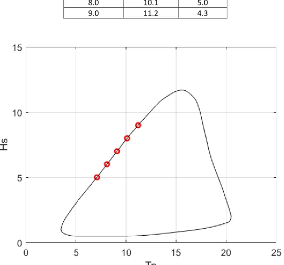
Sea states
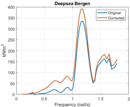
Additionally, wave power damping coefficients are estimated from the material in the Exwave Joint Industry Project, see Table 6-4. They were calculated for a common γ value of 3.3 and not the values in Table 6-3, but this is considered not to be a significant error in the simulations (considering that the damping of the DP system is one order is larger in size).
Simulations
- Parameter variation
- Simulation results
- Deepsea Bergen
- The Exwave semi
- Comparison of results fro the two semi-submersibles
- Probability of loss of position
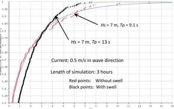
- Dependence of response on spectral peak period - probability curves
- Further analysis of results
Three-hour simulations were performed for Deepsea Bergen for the five sea states in Table 6-3. For movement, the standard deviations of the WF and LF parts are shown separately alongside the standard deviation of the whole movement (WF+LF). For the wave drift force in the table, the ratio is between 7.1 and 9.0, reflecting the fact that the force is exponentially distributed.
This further indicates that the Deepsea Bergen damping ratio is lower (Although Table 6-2 shows identical damping ratios for the two halves, these values are based on the mass-spring-damper analogy. Therefore the prescribed damping may deviate from true damping , which depends on how the filter delay and the drivers affect the characteristics of the control system. Also for the Exwave half, the response maximum is obtained for the second highest wave height. For the base case, the spectra are shown of wave motion force and surge motion in Figure 6-13 and Figure 6-14.
Study compound answers, e.g. transition motion, which may have a complex motion pattern that will include resonant roll and pitch motion. The drag force on the Deepsea Bergen piers was calculated for the same wave condition as in the pounding analysis. For the same wave condition, application of the Exwave formula has also been shown to result in a significant increase in force.
Simulations with the model for the Exwave semi and the five wave states give answers that are overall larger than those obtained with Deepsea Bergen. For the Exwave semi, the second largest significant wave height (8 m) produced a larger response than the 9 m significant height wave. The reason for this is the smaller wave period for the 8 m wave, as shorter waves will generally produce a larger wave drift force.
The probability of boundary crossing was calculated for the five wave modes on the 1-year contour.