Through space and time

Problem definition

Targeted Applications

Assumptions and Limitations

Methodology

Through this evaluation, we provided evidence of the system's performance and its compliance with the defined requirements. The use of quantitative methods allowed for a rigorous evaluation of the effectiveness of the system and the provision of measurable results.

Context

Contributions

Thesis Outline

We will also describe deep learning and the corresponding architectures of state-of-the-art models. The vertical extent of targets indicates the height of an object such as a school of fish or a scattered layer.

Stabilizing hydroacoustic data

Spatial filters

Frequency filters

Deep learning

• Neural Networks
• CNN - Convolutional Neural Networks
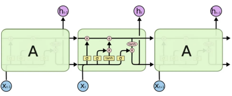
• RNNs and Transformers
• Transformers
• BERT - Bidirectional Encoder Representational Trans-

The self-attention mechanism calculates a weighted sum of the input sequence at each position. Positional coding of the input sequence was necessary to enable the model to use the order of the sequence.

ERS - Electronic Reporting System

The masked language modeling task is done by masking part of the input sequence and then predicting the masked input. This is done by choosing two sentences A and B, with a 50% probability of being the next sentence.

EchoBERT

The paper introduces a new task for echograms. Next time slice prediction is a task for the model to understand long-term dependencies in the echograms. The task of the model is to predict whether the vector is the true vector or substituted. The result of this task gives the model a two-way aspect with no mismatch between pre-training and fine-tuning.

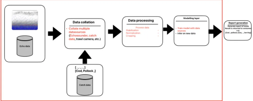
Machine learning pipelines

• CRIMAC
• Echo data processing
• Echo data stabilization
• Echo annotation
• Model Integration
• Data loader

Papers [15], [2] introduce the methods used for the preprocessing of data from the tobis survey. The candidate is selected based on the highest quality, which means the width and prominence of the folding peaks. The thesis' requirements derive from findings in the literature, as well as the context from section 1.5.

These files must be processed into a simpler, more interpretable form of data structure to easily adapt to new tasks. Moreover, it is crucial to consider computational overhead and efficiency in the context of collecting the echo data and capturing messages. The model integration should ensure seamless integration of the processed echo samples into the training pipeline, enabling efficient and effective model training.

The data loader component should be designed to load and process the data in batches efficiently.

Proposed Design

Processing Layer

Proposed model architecture and requirements

Objective function

Furthermore, the output layer of the model will be designed to change variably based on the label set or manually selected species. This flexibility allows the model to adapt to different scenarios where the number of target fish species may vary. The model will dynamically adjust the output dimension based on the input training data, ensuring compatibility with different label sets.

Loss function with temporal proximity weighting

Overall, the proposed model architecture will build on the strengths of the EchoBERT model, while introducing modifications to address the specific requirements of modeling fish abundance using hydroacoustic data. By incorporating switchable criteria, flexible output layers, and accounting for temporal proximity in the loss function, the model aims to provide accurate predictions and adaptability to different scenarios and label sets. Because each component's specific requirements and each layer in the pipeline must be presented individually, we will propose methods that explain how the design is implemented in our thesis and cover implementation-specific details.

To enable an iterative approach and quick evaluation of ideas, Python was chosen as the language for all components[21]. The language enables the use of a widely used package in the thesis domain, xarray[17], which enables parallel processing of labeled datasets. In this framework, both related work models were developed, their use in the diploma thesis became self-evident.

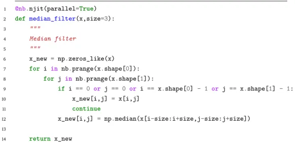
Finally, Number[22] was used to create embarrassingly parallel methods to facilitate the requirement for fast processing of echo and capture data.

Data processing layer

• Echo data processing
• Echo data stabilization
• Echo annotation
• Collation criterion

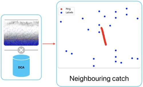
All multidimensional data objects generated from the database are written to disk to allow efficient retrieval and processing of catch data. After obtaining the catch data, the processing component performs a comparison of the echo data with the catch data object. This algorithm determines the distance within a given radius of hydroacoustic measurements, as shown in Figure 5.3.

In Figure 5.3, the points in blue are the neighboring catch messages within a 1𝑘𝑚 radius of the hydroacoustic coordinates (red). Since the Haversine method is applied for each index𝑖 ∈𝐴where𝐴 are vectors with latitude and longitude positions of the transect, denoted as𝐴𝑙 𝑎𝑡 and𝐴𝑙 𝑜𝑛 of magnitude𝑁. There is also 𝑗 ∈𝐵, which corresponds to the positional information from the catch reports, denoted as 𝐵𝑙 𝑎𝑡 and 𝐵𝑙 𝑜𝑛 of magnitude𝑀.

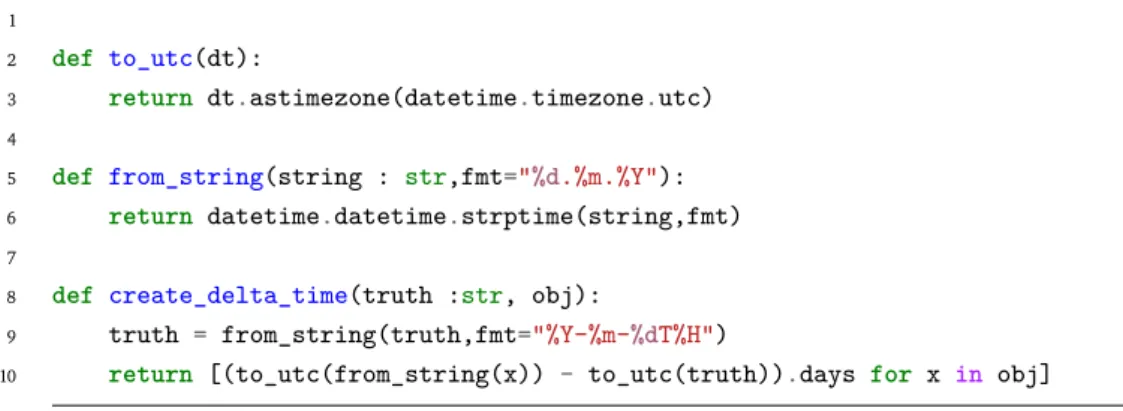
The code list 5 is the method to find all unique indices in the catch data, and the code list 6.

Model layer

Model integration and Data loading

The arrangement of the data is implemented by the related work EchoBERT[9] although the paper implemented the method for a continuous echo of the cages, the same principle is implemented in this thesis. The corresponding label for the selected threshold is read and converted into the desired label. We transform the labels into a stochastic distribution for the regression task or a multi-hot coded array for classification.

We have implemented methods for the multi-vector case that find all unique species codes for a corresponding threshold. This gives the model a naming set that corresponds to all existing species codes for the threshold. The final objective of the target transformation is to create data objects for temporal proximity weights.

The changes made compared to the original data loader are the method of retrieving samples from disk, the dimensionality of the data and the transformations as previously presented.

Model implementation

27 humbje = F.binary_cross_entropy_with_logits(preds, targets,weight=weight if self.temporal other Asnjë).

Temporal-proximity in truth labels

To investigate whether the catch messages are a good proxy for the abundance in an echo image, we compare it with an already annotated dataset. As presented in related works in Section 3.2.1, CRIMAC proposed several classification models for the sandpiper survey conducted by HI. For this thesis, we limit ourselves to one of the frequencies 128 kHz, since the gridding and adjustment of multiple back-scatters gives a higher logical complexity.

Benchmark setup

Experimental environment

Model parameters

Binary Model: The model output a single value representing the presence or absence of smaller sand eels. Multi Model: The model extracted all species in the label set for the different thresholds tested. Regression model: The model performed regression analysis, predicting the round weight distribution of smaller sand eels and potentially other species.

For each run, the data set was shuffled and split into a data partition, where the training data set was 0.8 and the validation and test set was 0.2.

Annotation experiments

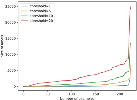
• Label size
• Unique species in labels
• Distribution of temporal proximity in data
• Computation Time of Catch and Echo Collation

This experiment is concerned with the number of unique species found in each label set for the different thresholds mentioned in section 6.4.1. The number of unique species present in each label set was determined by evaluating the annotation data using the specified thresholds (𝑇). This analysis provides insight into the diversity and distribution of species captured at different threshold levels.

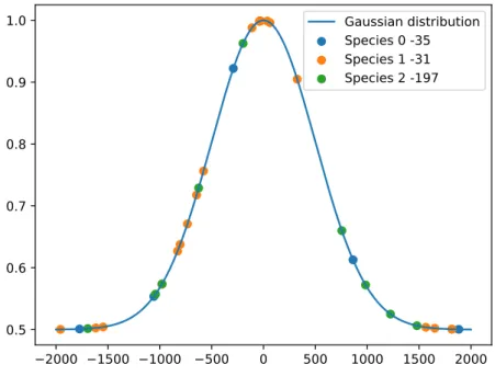
We examined the distribution of temporal proximity in the data to explore the potential of the weighted loss function. The spikes are about a year apart in days, indicating a repeating pattern in the catch data. The objective was to understand the relationship between the time required for the calculation of the distance matrix with different thresholds and the size of the found capture messages within the specified region.

The x-axis represents the time spent calculating the distance matrix, while the y-axis represents the size of the catch messages found within the region.

Model experiments

Regression method

Most of the processing times and sizes lie in the same quadrant of the plot, but there are external differences. The model classifies all classes as not present, while in reality, 25 of the classes are actually present. Temporal weighting is designed to assign different weights to differences between predictions and the ground truth based on the temporal proximity of species.

Pipeline design is based on theoretical considerations and preliminary field research. By using different or more frequencies, the model can capture more of the features of sand eels. The objective of the temporal proximity mechanism was to encourage the model to give more importance to the most recent samples during backpropagation compared to outdated labels.

Jech, “PyE-cholab: an open-source, Python-based toolkit to analyze water column sonar data,” The Journal of the Acoustical Society of America, vol.

Classification method

Preprocessing

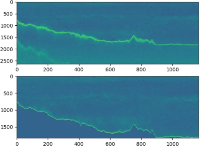
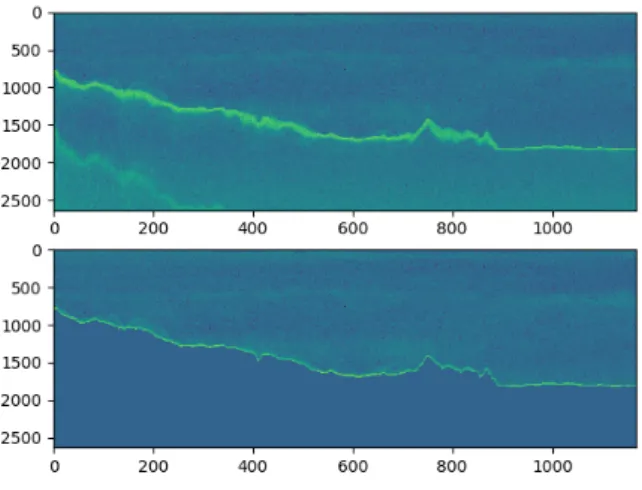
The test environment did not use the image cropping functionality based on subscripts, but instead segmented all features below the seabed to an intensity value of −90 dB. By cropping the seabed as shown in Figure 5.1, the patches of data sets would contain more relevant information while reducing the size of the data set. The sandstone survey data are already calibrated so that the backscatter shows a high signal-to-noise ratio.

However, noise filtering may become more important in field operations where echo sounders are not optimally calibrated. Preprocessing of .raw files used xarray datasets as the data structure, which offer convenient indexing capabilities for dimensions and variables, including auxiliary information.

Exploring the annotation

Label analysis

Label processing

An assumption made for the collector is that if the shape of the echo ping is greater than 6000, the sample will be skipped in the calculation. This was because the benchmark setup, with 72 cores and 256 GB of memory, started swapping memory access, resulting in a complete halt in the process.

Using the annotation

• Model dataloader
• Model analysis
• Processing layer
• Optimizing the model

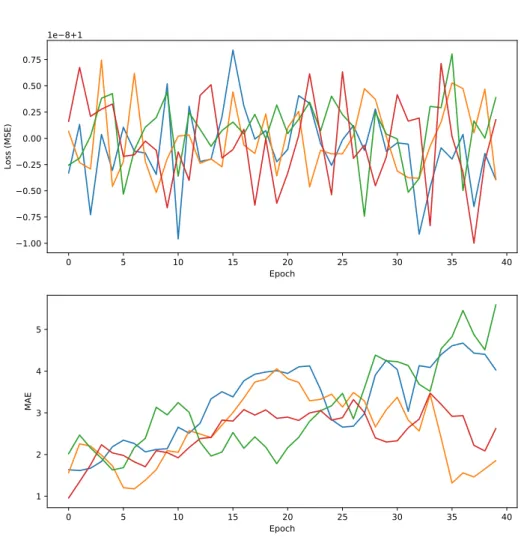
The loss function of the model is enriched and no patterns can be seen between the thresholds. The BCE is used as an objective function and the model indicates whether the selected species occurs in the ultrasound data. However, it is critical to note that while the assumption behind temporal weighting is true, the loss function used in the model is typically an average or the sum of all output neurons.

In conclusion, although the temporal weighting implemented in the model may not work as expected for the loss function, it can still provide valuable temporal information to guide the training of the model. The idea was to use the timestamps in the annotation to train the model based on proximity in time and proximity in the target target. Although the model may not have performed as expected, many propositions were constructed.

First, we can better understand the performance of the model using the F1 score on the test set, which takes into account precision and recall.