This thesis consists of studying and applying a new control structure at the Brobekk waste incineration plant. PhD student Johannes Jäschke at the Department of Chemical Engineering, who has been a great help during my work on this thesis.
M OTIVATION
This chapter gives a brief introduction to the structure of this master's topic, as well as an introduction to waste incineration plants.
S TRUCTURE OF THESIS
The Brobekk and Klemetsrud waste incinerators (WIP) are operated by the Waste Recycling Department of the City of Oslo (Energijenvinningsetaten), henceforth referred to as EGE. In 2007, new heat exchangers were installed, and later an air heater and frost protection system.
C OMPONENTS AT B ROBEKK
This thesis focuses on Brobekk, located in Alnabru, built in 1967 and was the first large-scale waste incinerator in Norway. This water comes from Hafslund Fjernvarme AS, henceforth referred to as Hafslund, which operates the district heating network in the city of Oslo.
O PERATIONAL ASPECTS OF B ROBEKK
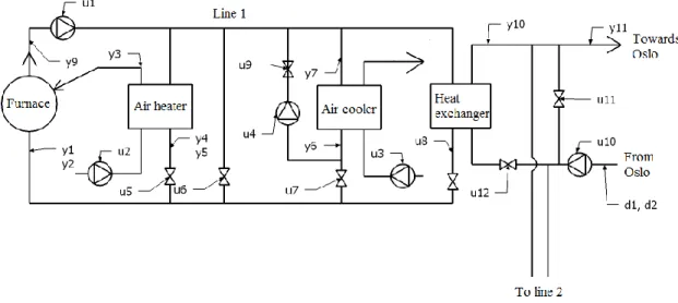
The flow rate can vary between 500 and 900 ton/h and is split equally between the two heat exchanger lines. If the heat needed from Hafslund falls below 32 MW, Brobekk must remove the excess energy using air coolers.
C URRENT CONTROL STRUCTURE
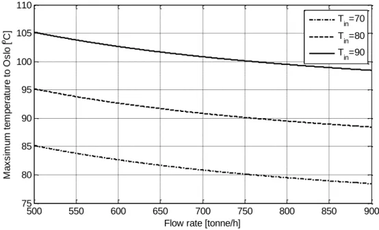
Water temperatures from Hafslund can vary between 65 and 90 °C, and water temperatures that Hafslund wants towards Oslo can vary between 95 °C and 110 °C. One of the biggest problems Brobekk faces is when Hafslund drastically reduces their flow to the heat exchangers due to less heat demand.
W ORK DONE BY H ELGE S MEDSRUD
Modelling
For the fans, Smedsrud uses the Bernoulli equation where he assumes a low pressure drop across the fan and a horizontal position. The Bernoulli equation is also used for the pumps, where the height is set to zero, the diameter is equal before and after the pump, and the pressure after the pump is assumed constant.
M ODIFICATIONS TAKEN INTO ACCOUNT IN THIS THESIS
Air heater
Since the system contains only pressurized water and non-compressed air, all thermodynamic and material properties such as heat capacities and densities were assumed constant and average values for the respective temperatures were used. Isothermal flow was assumed through pumps, fans and valves due to small pressure differences in the system.
Frost protection
Minor adaptations made to the model
This allowed the integral action in the PI controllers to be closed, causing some unintelligible simulation results.
I NPUT DATA TO THE MODEL
Predictive Control, or Model-based Predictive Control, MPC, is the only advanced control technique – that is, more advanced than standard PID control – that has had a significant and widespread impact on industrial processes (Maciejowski, 2002). The first part of this function is then used during a short time interval, after which a new measurement of the function is calculated for these new measurements. However, the earliest patent appears to be the one granted to Martin-Sanchez in 1976, who called his method simply Adaptive Predictive Control (Maciejowski, 2002).
But all these proposals shared the essential feature of predictive control; an explicit use of an internal model, the idea of a receding horizon and calculation of the control signal by optimizing future plant behavior. The next section provides a brief summary of the methods that can be considered the breakthroughs in model predictive control.
H ISTORICAL DEVELOPMENT
LQG
Solving this problem involves two steps; first, the measurement of outcomes y at time k is used to obtain an optimal state estimate xˆk k|. The LQG controller has good stabilizing properties; given that the internal linear model is almost identical to the real plant. A major drawback to the LQG controller is that it does not handle input and state constraints.
M ODEL PREDICTIVE C ONTROL
- The objective function
- Internal model
- Control interval
- Prediction horizon
- Control horizon
- How to choose good interval and horizons
- Constraints
- Infeasibility
- MPC Tuning
- Square plants and non square plants
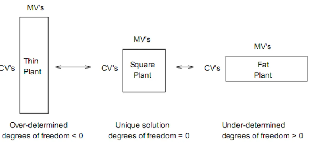
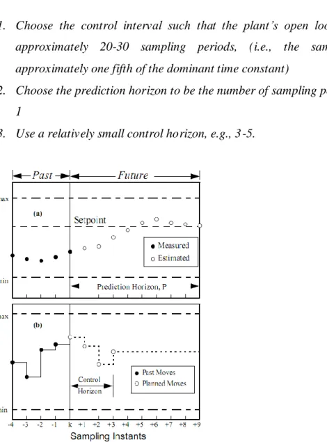
The control horizon is the number of future optimal control moves calculated at each sampling time. Choose the control interval so that the open-loop settling time of the device is about 20-30 sampling periods (ie, the sampling period is about one-fifth of the dominant time constant). In a "thin" plant, there are not enough inputs to meet all the control objectives, and the outputs are free to move.
The control specification must be relaxed or the resulting violation can be minimized in a mean square sense (Qin & Badgwell, 2003). In the square plant, the quantity of inputs equals the quantity of outputs and the MPC is able to meet the control objectives.
N ONLINEAR MPC
C ONTROL STRUCTURE
If an MPC is used at the supervisory control layer, a regulatory layer is not required because the MPC is able to directly control physical inputs. Another alternative is to have the MPC at the supervisory layer control set points for the regulatory layer. The stability and performance of a lower (faster) layer is not greatly affected by the presence of upper (slow) layers due to the frequency of the "disturbance".
With the lower (faster) layer in place, the stability and performance of the upper (slower) layers does not depend much on the specific controller settings used in the lower layers because they only affect high frequencies outside the bandwidth of the upper layers. The thesis will focus on the lower layers in the control structure, so the higher layers will not be considered in this thesis. a) MPC controls setpoints for lower layer controllers.
C ONTROL CHALLENGES OF HEAT EXCHANGERS
As mentioned in the problem description, one of the tasks was to investigate whether it would be worthwhile to apply an MPC or a non-linear MPC for controlling the real installation. However, in this thesis it was decided to use MATLAB's Model Predictive Control Toolbox, a linear MPC. The model developed by Smedsrud was created in Simulink, a supplementary package to MATLAB.
The Model Predictive Control Toolbox provides Simulink blocks and MATLAB functions for designing and simulating model predictive controllers, both in MATLAB and Simulink. The remainder of this chapter presents the various MPC alternatives designed for the Brobekk waste incinerator model, and hopefully the results can be valuable to solve the problems described in Chapter 2.2.
MATLAB MPC T OOLBOX
Optimization problem
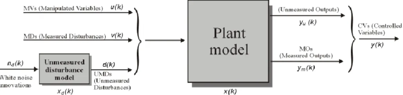
Prediction Model
C ONTROL CHALLENGES AT B ROBEKK PLANT
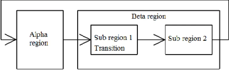
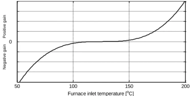
Alpha region
Beta region
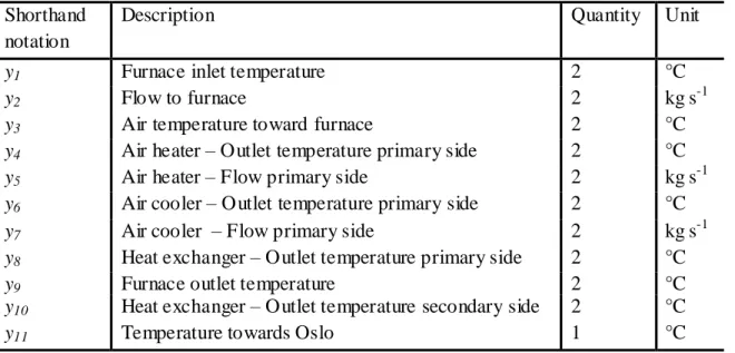
The first sub-region is when the outlet temperature of the primary side of the air cooler, y6, and the outlet temperature of the primary side of the heat exchanger, y8, are lower than the inlet temperature of the furnace, y1. This subregion is described by the air cooler primary side outlet temperature, y6, higher than the furnace inlet temperature, y1, and the heat exchanger primary side outlet temperature, y8, lower than the furnace inlet temperature, y1. In the third subregion, the cooling air primary side outlet temperature, y6, is lower than the furnace inlet temperature, y1, and the heat exchanger primary side outlet temperature, y8, is higher than the furnace inlet temperature, y1.
The fourth subregion when the air cooler main side outlet temperature, y6 and the heat exchanger main side outlet temperature, y8 are higher than the furnace inlet temperature, y1. When moving from region α to region β, it will be more reasonable to force the process to sub-region 2, because the temperature of the main outlet of the heat exchanger is already lower than the temperature of the furnace inlet.
C ONTROL STRUCTURE DESIGN
PI controllers
The steady-state gain k and time constant τ1 were obtained using the step responses and then approximating a first-order transfer function model. The tuning parameters for the PI controllers were then found using Skogestad/Simple Internal Model Control (SIMC) (Skogestad, 2003). 1 The controller parameters for the main flow controller had to be reconfigured because the SIMC gave too high a controller gain.
At the time 8000 sec. the temperature regulator in the frost protection system begins to stabilize the temperature at 10°C. The set point for this flow is 250 ton/h, which is in line with the operational aspect at Brobekk.

MPC design - Alpha region
MPC design - Beta region
S IMULATIONS
Alpha region
The heat exchanger valve and the cooling air fan and valve were weighted with large weights to prevent these manipulated variables from drifting away from the set value. The set point was set to one for the heat exchanger valve and zero for the fan and cooling air valve. And it can be seen that the outlet temperature of the heat exchanger never reaches the temperature that Hafslund wants.
The heat exchanger valve is almost fully open all the time while the bypass valve is used to control the furnace inlet temperature. The small drops in the heat exchanger valve are because the valve is not weighted enough compared to the other variables.
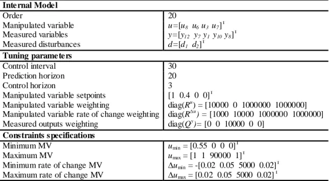
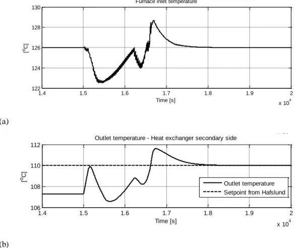
Beta region
In addition to the heavy weight on the furnace inlet temperature, heavy weight was placed on the secondary heat exchanger outlet temperature. As can be seen from Figure 6.12 (b), the side outlet temperature of the secondary heat exchanger follows its set point well. The bypass valve at Hafslund was closed during the simulation, so the temperature shown in Figure 6.12 (b) will be the temperature towards Oslo.
The side outlet temperature of the secondary heat exchanger varies even more and the deviations are somewhere around 7°C. The flow varies greatly and this again affects the furnace inlet temperature and the main side outlet temperature of the heat exchanger.

Transition from alpha to beta region
When the heat demand from Hafslund falls below 32 MW, the plant enters subregion 1, and thus the MPC developed for this region is used. When the air cooler primary side outlet temperature goes above the furnace inlet temperature, the control system enters subregion 2 and switches to the MPC developed for this region.
Transition from beta to alpha region
Considerations of the different MPCs developed in this thesis; it appears that they all offer promising control over the inlet temperature of the furnace and the outlet temperature on the secondary side of the heat exchanger. In alternative 1 for the β region, the control structure developed here seems to promise good control of both the inlet temperature of the furnace and the temperature towards Oslo, thus meeting the requirements of both EGE and Hafslund. In alternative 2 for the β region, it was found that the bypass valve on the Hafslund side disturbs the temperatures in Brobekk, causing more variations in the furnace inlet temperature.
This can reduce the variations in the furnace inlet temperature and the secondary outlet temperature of the heat exchanger. But it is unknown how "slowly" the bypass valve must be set, and probably the performance will not be better than in alternative 1. Overall, it is concluded that the proposed control structure controls the system very well when EGE only controls valves on the Brobekk side of the heat exchanger.