The study summarizes relevant previous work and characterizes the expected random and systematic errors encountered when surveying with standard MWD in the Barents Sea. The study summarizes relevant previous work and characterizes the expected random and systematic errors encountered in MWD surveys in the Barents Sea.
INTRODUCTION
- Background
- Problem Definition
- Regulations and Standards for Directional Drilling
- The Activities Regulations
- NORSOK D-010
- Scope of Work
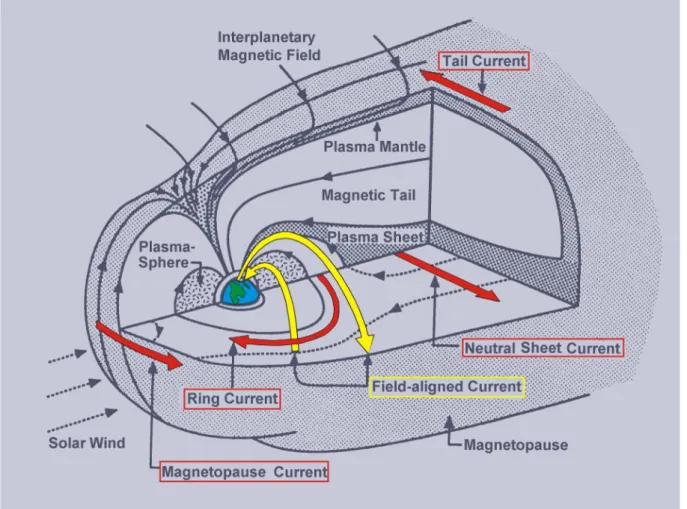
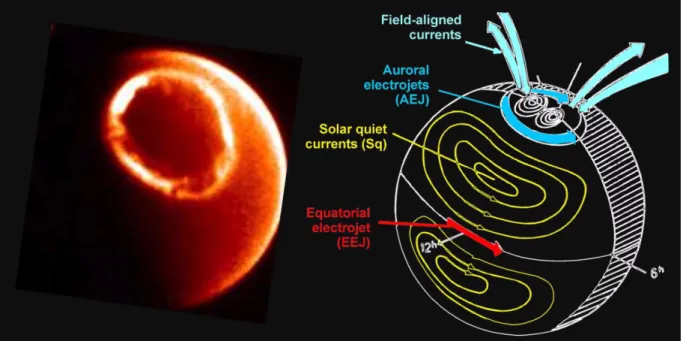
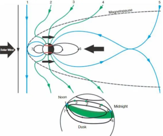
Currents in the ionosphere are present even during quiet times and are caused by tides of the atmosphere. Finally, any time-varying disturbances in the magnetic field cause electric fields in the Earth and oceans.
MEASUREMENT WHILE DRILLING
- General
- Directional Drilling
- Well Placement
- Magnetic Surveying Instruments
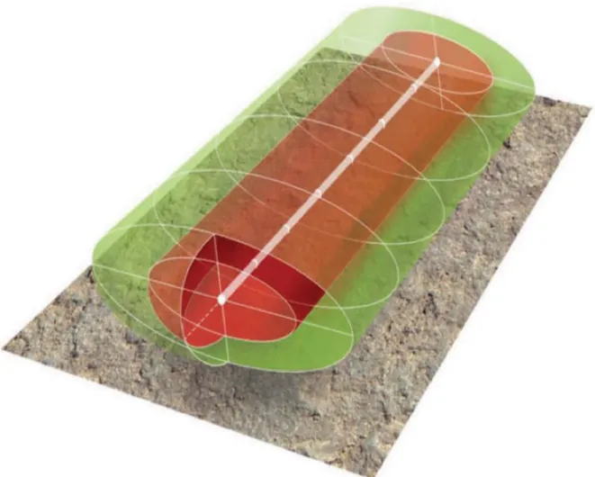
- Ellipses of Uncertainty
- Collision Avoidance
- Geological Targets
- Relief Well Drilling
- Global Field Models
- Crustal Anomaly Mitigation
- Disturbance Field Mitigation
Any interference in the horizontal-east/west direction relative to the reference model will result in corruption of the survey azimuth. Distance instruments also rely on detecting small disturbances in the magnetic field to identify the location of the well casing.
CHALLENGES WITH MWD MEASUREMENTS IN THE BARENTS SEA
Thus, the external magnetic field variations in the Norwegian Sea and Barents Sea areas were studied with special attention to the declination (Edvardsen et al, 2013). Given these challenges unique to the region, the approaches presented in the sections that follow provide critical fixes to operations in the Barents Sea and corresponding risk mitigation.
MITIGATION METHODS
General
Crustal Anomalies and Mitigation
- In-Field Referencing
- Aeromagnetic Surveys Available for IFR in the Barents Sea
- Barents Sea Study
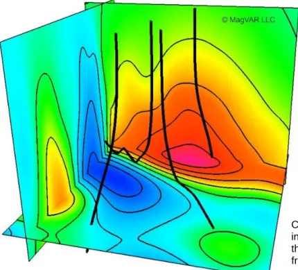
Outside the grid region, we assume a typical long-wavelength crustal anomaly with 400 nT amplitude (red in Figure 4.1). Finally, 𝑔𝑛𝑚 and ℎ𝑛𝑚 are the ellipsoidal harmonic model coefficients of the expansion, estimated by least squares from the input data for the area. A detailed validation study of the ellipsoidal harmonic IFR algorithm was published by Poedjono et al (2012).
The IFR values calculated using the Flat Earth method are approximately twice as large and do not meet the ISCW assumptions. This is because the line spacing directly affects the lower limit of the range of wavelengths that can be captured by the survey. More recent surveys of the southern Barents Sea were carried out by NGU with a line spacing of 2 km (Table 4.2).
A buffer of at least 10 km from the edge of the input data must be included to avoid edge effects. Areas of the Norwegian Sea are surveyed in this detail and a tighter spacing can further improve the uncertainties shown using the ellipsoidal harmonic method.

Geomagnetic Disturbance Field Mitigation Study
- Global Climatological Models of Magnetic Disturbance
- Prior Work - Nearest Observatory
- Real-Time Local Observatory
- Interpolated In-Field Referencing
- Disturbance Function
- Barents Sea Simulation Study
- General Findings
In general, to reduce the disturbance field by 75 % (in other words, to get to 25 % residual error) requires an observatory within about 60 km of the drill site, as illustrated in Figure 4.8 below. The real-time local observatory method involves placing a physical magnetometer within a few km of the drill site. The surrounding observatories may not be ideally located on both sides of the drill site.
In fact, these changes in the disturbance field are used in the geomagnetic depth sounding method to map subsurface conductivity. DF addresses both issues by first deploying a mobile observatory at a land or bottom ocean location in close proximity to the training site. Any modulation in the amplitude and phase of the disturbances between the observatory and the training site is then optimally accounted for.
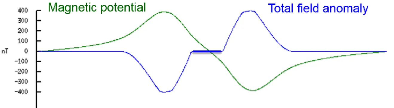
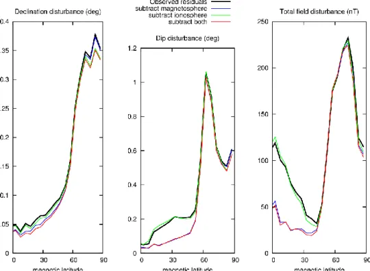
Specifically, we were interested in comparing how much of the perturbation field could be reduced with the various mitigation methods available. This is illustrated in figure 4.17 by the larger bumps on either side of the peak.
RESULTS AND DISCUSSION
Wellbore Uncertainty in the Barents Sea
- Prototype Well
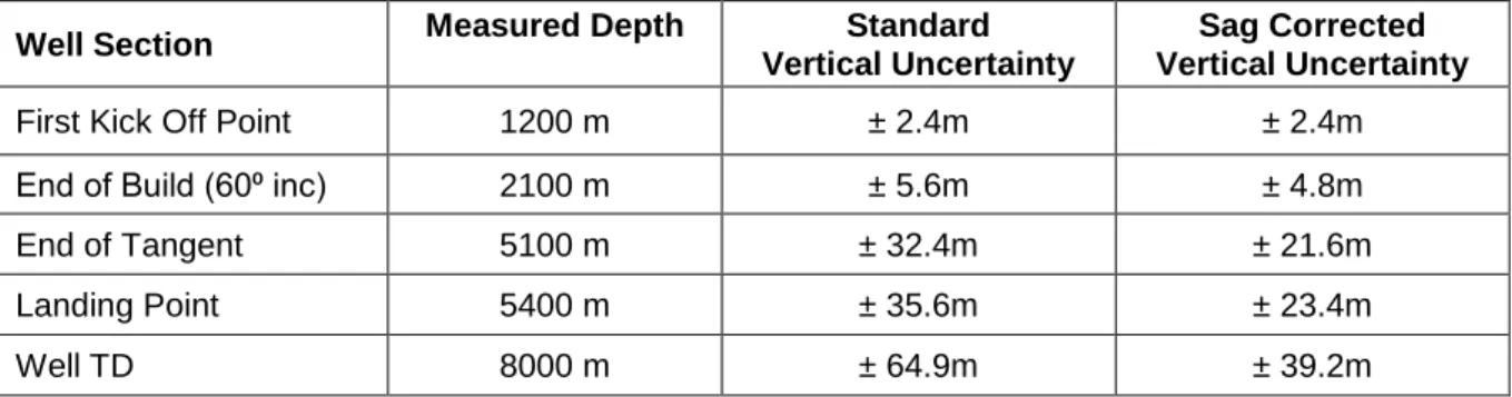
- Vertical Uncertainty
- Lateral Uncertainty
- Uncertainty Reduction Considerations
Changing the magnetic reference values used to correspond to those expected in the Barents Sea. Further reduction of the declination error can be achieved by taking local magnetic measurements and building a high-accuracy model of the crustal field in the area to be drilled. This process known as Type 1 Field Referencing (IFR1) can greatly reduce lateral uncertainty in the wellbore, especially in the North/South direction.
The presence of magnetic components in the bottom hole assembly will create an effective bias on the axial magnetometer in the MWD sensor. At the high latitudes such as those represented in the Barents Sea, the magnetic disturbance field is a confounding factor when attempting to apply multistation analysis. It should be noted that these ranges are generally lower than the estimated relative uncertainties modeled in the exchange scenario above.
There are several techniques that can be used to increase the capabilities of the various instruments in the emergency well scenario. The uncertainty of the wells is low enough to establish remote contact and reduce the relative uncertainty in the wells to a manageable level.
Effects of Inaccurate Geomagnetic Referencing
- Dominant Errors and Directional Dependence in MWD Surveying
- Drillstring Interference Observability and Survey Corrections
- Ensuring the Quality of Multi-Station Analysis
- Reference Error Simulations
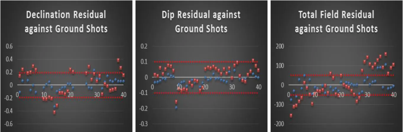
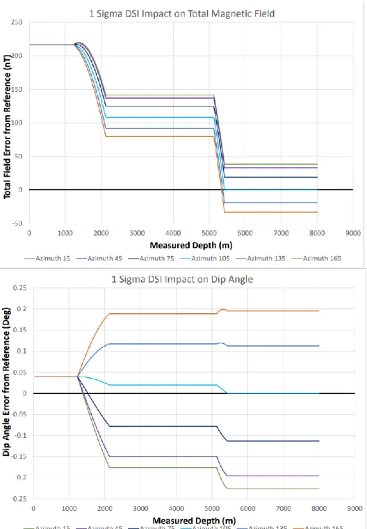
The graphs in Figure 5.4 show a model of how drillstring interference at the 1-sigma level for the MWD standard error model (220 nT) is expected to affect the overall magnetic field and dip measurements for each of the sample wells. The trends in these field acceptance criteria closely follow those of the modeled drill string interference from Figure 5.5. Instead, a mathematical transformation can be performed that directly integrates the covariances of the quality control parameters and assigns each measurement a relative error (known as the Mahalanobis distance) with respect to the expected reference.
The presence of any errors that are not aligned with the borehole axis (such as cross-axis sensor biases or geomagnetic reference field errors) will violate the assumptions of the corrections and add errors to the survey azimuth. Crustal anomalies will cause systematic deviations in the magnetic measurements relative to the modeled reference values, not unlike the effect of drill string interference when drilling a straight section of the wellbore. An example of the raw recording quality control measurements together with the post-correction quality control is shown in Figure 5.7 and Figure 5.8.
Each of the raw surveys would have been equally accurate, having been corrupted by the same amount of drill string interference. The accuracy of corrected surveys is directly related to the quality of the drill string interference estimate.
Discussion
- Crustal Mitigation Results
- Disturbance Mitigation Results
- MWD Note
Of these two methods, the ellipsoidal harmonic method was found to be most likely to meet the requirements of the OWSG MWD+IFR1 fault model, as long as aeromagnetic data of at most a 4 km line spacing is available. A data search was conducted which found that aeromagnetic data of this quality were present for the western part of the Barents Sea (west of 32 ⁰ E longitude). To determine line spacing of data available for a particular sub-region of the Barents Sea, one can refer to Figure 4.5 and Table 4.2.
The current data search found data, but not of sufficient quality for an OWSG IFR1 compatible model that also covers the eastern part of the Barents Sea. Of these three methods evaluated, the perturbation function method achieved the best prediction of the local magnetic values, especially as the distance to the nearest magnetic observatory increases. Because geomagnetic latitudes in the Barents Sea are in the mid to high sixties, 68° is chosen as representative.
The effect of the crustal and perturbation fields on the ability to control the quality of MWD data was studied. Of primary interest is the impact of the perturbation field on raw quality control measurements for MWD data.
RECOMMENDATIONS
General Recommendations
Specific Recommendations Resulting from this Study
In the western part of the Barents Sea (west of longitude 32°E), IFR1 can be easily implemented with the available data to meet the requirements of the MWD+IFR1 tool code. In the eastern Barents Sea (east of longitude 32°E), higher resolution magnetic data (maximum 4 km line spacing, ideally 1-2 km) will be required to meet MWD+IFR1 requirements. This may already be available for discovery or acquisition, or a new high-resolution aeromagnetic survey may need to be conducted.
Seabed magnetometers should be used for any operation where cost is not an issue and the utmost accuracy is required. In regions of the Barents Sea within ~50 km of a magnetic observatory (e.g. near the coast), the Disturbance Function method can be used to meet IFR2 tool code requirements. It is possible that the Nearest Observatory method or IIFR could also be used, but if these are applied a local survey should be carried out prior to drilling to confirm that uncertainties are within the IFR2 tool code.
In regions of the Barents Sea between ~50 and ~250 km from the nearest magnetic observatory, the Disturbance Function method must be used to meet IFR2 tool code requirements. In remote areas of the Barents Sea, further than ~250 km from the nearest magnetic observatory, a local magnetometer (seabed or otherwise) with real-time datalink must be deployed to meet IFR2 requirements.
34; Model-observation comparison for the geographic variability of the plasma electric drift in the Earth's innermost magnetosphere." Geophysical Research Letters (2017). In the first step, a rigid corotation of the ionosphere with the solid Earth was assumed in the model. 34; Confidence limits associated with values of the Earth's magnetic field used for directional drilling." In SPE/IADC Drilling Conference and Exhibition.
34;A corotational model of the Earth's electric field derived from Swarm satellite magnetic field measurements." Journal of Geophysical Research: Space Physics. Abstract: In a borehole measurement (MWD), borehole azimuth is determined relative to the direction of the geomagnetic field. The direction of the geomagnetic field in the auroral area can change by several degrees in less than an hour.
Representation of the local crustal magnetic contribution is critical to the process, as it represents a significant error in the position of the lateral borehole. E., “Extending comprehensive models of the Earth's magnetic field with Ørsted and CHAMP data.” Geophysical Journal International.
APPENDIX - TECHNICAL NOTES AND PREVIOUS WORK
- General
- Positional Error Models
- Solving MWD Challenges With IFR
- Creating An IFR Model
- Case Study In Disturbance Field Mitigation
- The Disturbance Function Method
- Remote Observation Through Land & Seafloor Magnetometers
A better understanding of the natural variations in the local magnetic field is essential for the successful development of the field (ibid). In the project described in the successful use of geomagnetic referencing to accurately determine the position of a well in a deepwater project offshore Brazil (Poedjono et al. 2012), the collaboration between the operator, contractors and academic experts and the development of a high-resolution geomagnetic model (HDGM) National Geophysical Data Center USA improved the spatial resolution to 30 km. However, according to Maus et al. 2017), creating an IFR model requires capturing the full spatial wavelength spectrum of the geomagnetic field.
Perturbation field mitigation was employed to monitor and correct directional surveys at the Haltenbanken area of the Norwegian Sea over a period of approximately 2 years with an increasing number of geophysical observing stations in Norway and Denmark, maintained by the Tromsø Geophysical Observatory (TGO) ( Edvardson et al. 2013). These techniques have become increasingly feasible due to the development of the Seabed Electromagnetic Station (SFEMS) (Toh et al. 1998, Toh et al. 2010). This gradient must be subtracted from the data before the residuals are treated as time variations of the total magnetic field.
The data in Figure 8.2 show the estimated crustal gradient after being removed from the measured data to recreate temporal variations in the disturbance field. Much like in the aforementioned Haltenbanken area in the Norwegian Sea (Evardsen et al. 3013), these time-dependent current fluctuations in the Earth's ionosphere cause inaccuracies in wellbore directional surveying, which only increase at higher latitudes.
ACKNOWLEDGEMENTS