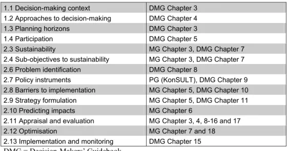
For each of the objectives set out in the Guide for Decision Makers, performance indicators will need to be drawn up. The relationship between the Methodological Guide and the third of the PROSPECTS guides, the Policy Guide, is quite different.
The decision-making context
Approaches to decision-making
Planning horizons
Participation
Plan-based and consensus-based approaches can be combined by setting goals and objectives through initial discussions and by inviting public participation at various stages of the planning process. The need to communicate with stakeholders must be reflected in the planner's work.
Summary
In many cases it is now defined as part of the planning process, and in some states it is required by law. It is important to consider carefully what level of participation is appropriate and why participation is desired.
The scope of our planning
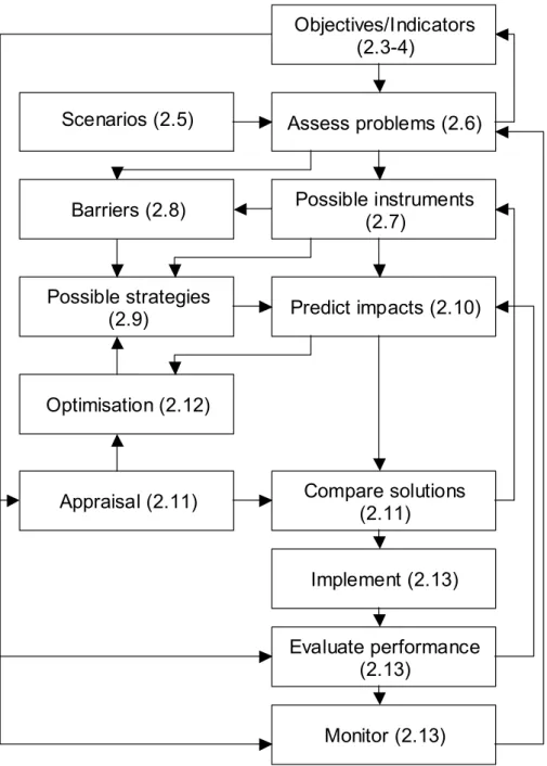
A logical structure
It provides a means to assess whether the implemented instruments have performed as predicted, and therefore enables improvement of the models used for forecasting. The scenario description (Section 2.5) forms a basis for problem identification, modeling and assessment and is vital for uncertainty analysis.
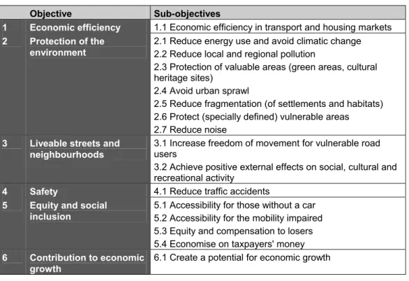
Sustainability – the basic objective
Sub-objectives to sustainability
A permanent body to monitor the implementation of the long-term plan would probably contribute to increased consistency between the long-term and short-term plans. It will then be possible to decide on the relative importance of the objectives on our suggested list.
Scenarios
Problem identification
Policy instruments
Barriers to implementation
Strategy formulation
Predicting impacts
Appraisal and evaluation
Optimisation
Implementation and monitoring
A land use and transport strategy consists of a combination of tools of the types set out in Section 2.7 and listed in Appendix I. Such analyzes are often aided by using a model of the land use and transport system.
Summary
This chapter sets out a consistent and flexible framework for evaluating urban land use and transport strategies that can be useful for all strategic planning for urban sustainability. Rather, the intent is to provide ideas for improving the methods used within such frameworks to account for specific assessment issues encountered in integrated urban land use and transportation planning for sustainability.
The appraisal framework
Thus, on the one hand, Table 3.1 provides information on the overall result with the weights that the analyst used to add up the individual impacts. The most important distributional impacts from Table 3.1 are included by introducing several rows in Table 3.2.
The main purpose of appraisal
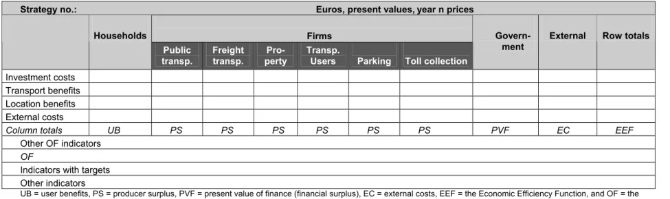
Transportation Benefits Locational Benefits External Costs Column Totals UB PS PS PS PS PS PS PVF EC EEF. UB = user benefits, PS = producer surplus, PVF = present value of financing (financial surplus), EC = external costs, EEF = the Economic Efficiency Function, and OR = the Objective Function, which consists of a linear combination of the EEF and other indicators.
Sustainability objectives and indicators
These are process indicators, not outcome indicators, in the terminology of the Decision-Makers' Guidebook. For example, it may be that parts of the benefits are ultimately reaped by agents outside the city.
Forms of appraisal
Note that if there are targets for indicators that are not included in the objective function, the assessment will include both the objective function score (actual number) and an assessment of whether the remaining indicators' targets have been met (yes/no or possibly the level of target attainment). Assign weights to each of the criteria to reflect their relative importance to the decision.
Measuring sustainability
Together, these elements form what we might call the core of the objective function — the first sum of terms. We can now enumerate the possibilities regarding indicators that are not included in the core part of the objective function.
Taking uncertainty into account
In conclusion, we do not need to include all indicators as parts of the objective function or as objectives in the optimization problem. This is the real choice approach (Dixit and Pindyck 1994), which also requires probabilities for the scenarios.
Presentation to decision-makers and the public
Even more importantly, the presentation of the results can be done at different stages of the planning process, from the early results of the first exploratory tests to help formulate the strategy, to a final report, structured according to the rules and national regulations. Each presentation may have its own purposes, including of course the purpose of providing decision makers with the information they need to rank or choose between strategies, but perhaps also the purpose of inviting ideas for further testing or the purpose of raising awareness of the issues in question.
Presentation to professionals
To draw conclusions from the results about what options exist and what normative and positive assumptions drive the results would be even more important. The presentations for each group will have to be different, both in terms of content and presentation techniques.
Presenting the individual indicators
Indicators of livable streets and neighborhoods can be a subgroup of the accident indicator, namely accidents involving pedestrians and cyclists. This helps a layperson (decision maker and public) to quickly grasp the main points of the presentation.
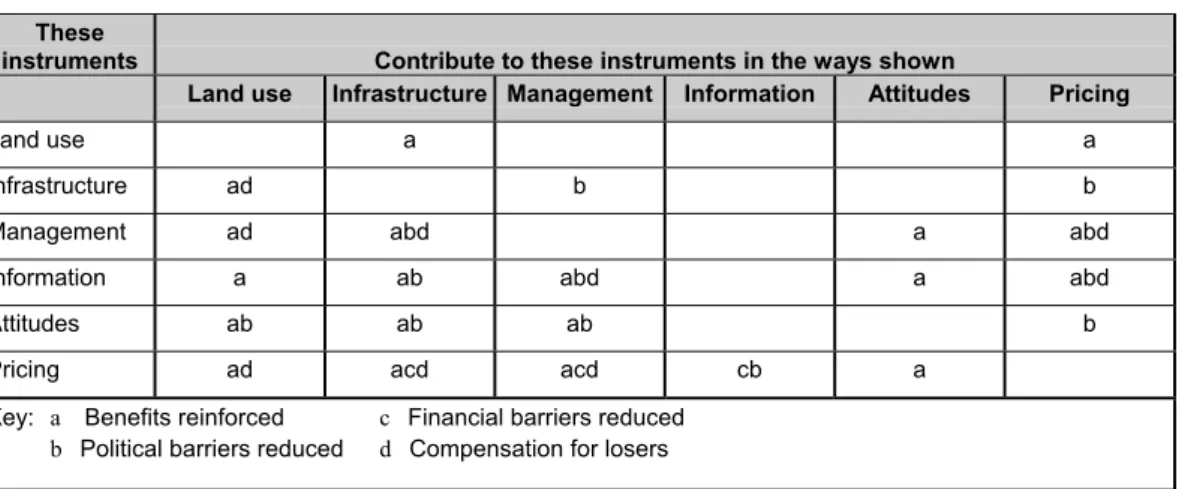
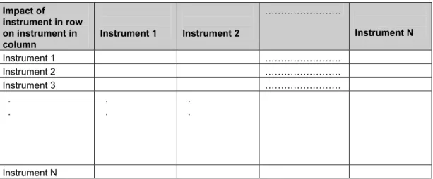
Analysis of synergies
The Institutional Responsibilities Matrix indicates, for each pair of instruments, whether the same institution is responsible for both instruments, and if not, the specific institutional differences involved. A public authority (or agency) is responsible for one instrument and the private sector is responsible for the other instrument.
Financial barriers
If so, it is necessary to report in the integration matrix only those factors that are considered most important. Removing this barrier must mean that the city does not have to repay its loans during the assessment period (which is clearly an unsustainable practice if the assessment period is long), or it means that money continues to flow into the system from outside sources, in any degree. Required.
Introduction
With the coding done, it's up to the model's logic to figure out what the implications are. To return to the confusion surrounding the concept of model, it is the logic in box F above that is the model.
The need for models
If the system in question is complex, it may be useful to view it as made up of different subsystems, each treated with its own submodel.
What is a good model?
Lundqvist and Mattsson (2002) discuss the issue of model validation in the context of national transport model packages. Verify that the system level model package is well designed and applied to the problem: are the right things exogenous/endogenous in the models.
A quilt of theories
It is also possible to derive the gravity model from information minimization assumptions (see e.g. Snickars and Weibull, 1977). An interesting point is that the multinomial logit (MNL) model can be derived from both random utility maximization and information minimization/entropy maximization, as shown by Anas (1983).
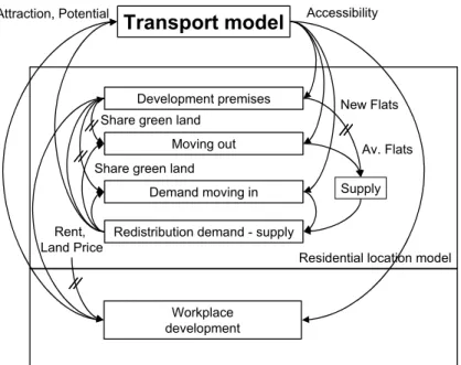
Land use-transport interaction (LUTI) models
There is currently much debate in the research community about the relative advantages of system dynamics and equilibrium approaches. AGAINST A systems dynamics model is overly dependent on the accuracy of the parameters it uses: if these are inaccurate, the model can go in strange directions and produce unbelievable or wrong results.
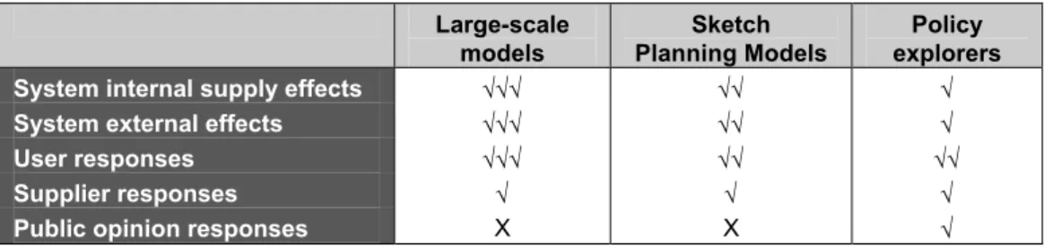
Sketch planning models
Policy explorers
The forecasting model at the heart of PLUTO represents all the main mechanisms that influence the development of the land use and transport system in real cities. For the purposes of the exercise, users can therefore assume that Plutopia is a real city and behave accordingly.
Desired capabilities
Because of the difficulties in predicting these responses, they are often modeled as changes in the input assumptions. In light of the current trend of liberalization of transport markets and the ongoing lack of coordination of land use and transport responsibilities in many cities, this is a shortcoming of current model systems.
Background
The local instruments must be assessed within the overall framework in relation to the common set of indicators (as described in chapter 3). Alternatively, the instrument can be considered without constraints within the optimization process and the benefit of removing the barrier can be presented to the decision maker.
The general optimisation problem
Targets for some of the indicators can also be modeled as constraints in the optimization problem. We have seen that it is important to recognize that there may be barriers to the use of the policy instruments.
Optimisation approaches
The calculation of the objective function is based on the results of both years and the shown interpolation of benefits. Some optimization algorithms require the value of the derivative of the objective function for arbitrary values of the function arguments.
Introduction
The elements of the economic efficiency indicator
Transfers cannot be ignored or eliminated too quickly in the calculation of economic efficiency. The government column can be multiplied by a shadow cost of public funds to reflect the fact that taxes create inefficiencies in the economy.
Discounting
If the covariance is 1 (annual earnings and national income appear to move closely together), the risk premium is set to 4.5%, which implies a discount rate of 8%. For strategies that deliver the same returns regardless of economic conditions, the risk premium is 0.
A multi-modal analysis
Therefore, finding the appropriate discount rate to use in a cost-benefit analysis is not straightforward. For example, official guidance in Norway (Finansdepartementet 2000) is to use a risk-free rate of 3.5% and add a risk premium depending on the covariance.
Introduction
Need for alternative to the traditional rule-of-a-half formula
Broadly speaking, we can identify the improvements not reflected in the generalized costs as land use benefits. It is clear that land use benefits, if they occur, cannot be captured by the traditional "rule-of-a-half" measure of user benefits.
Consistent benefit calculation in some types of model
If, on the other hand, we use the benefits from the land use model in this case, another part will be missing, namely the benefits in the transport system, which were not included in the land use model. But we would never be able to capture benefits from improvements in the destination zones (such as higher wages).
User benefit formulas in a logit residential choice model
The "A" terms can be calculated from a transport model, whereas the other terms require a land use model of the form (9.4).22. The agricultural model's Ai can consist of a sum of such Ai**pt.
The effect of requiring housing market equilibrium
H is the number of residents, U is utility from home-based activity minus rent, R is an index of environmental quality in the residential zone, f relates to the size of the zone and the alphas are constants (see the text in section 9.4). Like the elements of Vi, the shadow period will appear as a separate term in the half-rule formula.
On landlords, rents and shadow rents
User benefits must then be calculated with these additional shadow lease terms included. If the shadow interest rate does not change from situation 0 to situation 1, this term disappears.
The underlying theory
These shadow prices are probably model production. If not, it will be a difficult task to adjust the shadow prices so that the Hi of each zone remains within the constraint).
Be cautious, use judgement!
Second, it is perfectly legitimate and accurate to decompose this measure and calculate the benefits in each travel market using the aggregate demand functions and a linear path from the base case to the policy case—that is, using Hotelling's generalized profit measure. with the simplest possible path. Changes in the location of homes and the consumption of housing services are predicted in the model part of the land use of the modeling system.
Introduction
Example of presentation of economic efficiency results according to sectors and other indicators No. Strategy: Euro, current value, prices of year n. Investment costs Transportation benefits Location benefits External costs Column totals UB PS PS PS PS PS PVF EC EEF Other OF indicators.
The first element, (WTP – P)
The second element, (P – SC)
Thus, the private costs of production are changed into real social costs by adding the external costs imposed on others. Of course, we can disregard external production costs in the case of a good in fixed supply, but the transfer of use from one person to another can be different from the external costs arising from the use of the good).
Practical rules
There is, of course, an element of the correction period that must be entered into the government account. All other goods taxes on inputs (perhaps mainly fuel taxes) should be posted to the government account.
Summary
Since they can reclaim VAT and business trips are never final consumption, the rules for entering taxes and charges in the social accounting are exactly the same for business trips by public transport and for freight transport. How to enter taxes and levies in the government and carrier columns should be clear from table 10.2.
Definition
Producer surpluses of operators
Next, the total number of vehicle hours must be multiplied by labor costs per hour to give the time-dependent operating costs. Finally, the preparation costs and the remaining parts of maintenance and insurance depend on the number of vehicles in operation during a day.
Government surplus
Based on such information, the total number of vehicle kilometers in operation per vehicle type is assessed, which must be multiplied by the energy cost per kilometers to give the distance-based cost. The total number of vehicles (of different types) needed to run the peak schedule determines the rolling stock cost, which is another type of time-dependent cost.
Environmental and safety impacts, overview
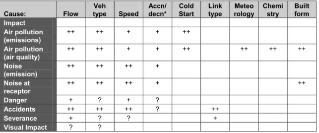
The second factor is the change in the level of impact from the "to-minimum" baseline condition; again, severity may be monotonically related to the degree of change, or thresholds may be used. Strength of influence of factors affecting the environment and disasters Factor: Absolute level Threshold Change Connection type Built form Impact.
External costs in the economic efficiency indicator
Conventional network models outperform this slightly in that they estimate speed per link, thus providing more accurate estimates of impact. Microsimulation models can estimate acceleration and deceleration levels directly, but are too detailed to assess city-wide strategies.
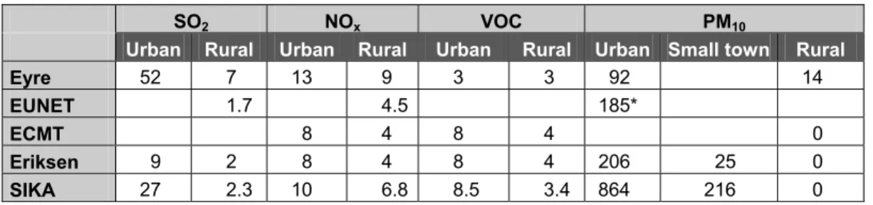
Calculation of environmental costs
Improvements in fuel efficiency and cleaning technology and changes in the composition of the vehicle fleet will obviously matter for the emission factors. Estimates of life cycle costs of manufacturing cars and houses can also be found in the literature.
Calculation of accident costs
When it comes to assigning walking and cycling trips to zones, there seem to be two main options. The research shows that research is needed to better capture the benefits of walking and cycling.
Aspects of equity
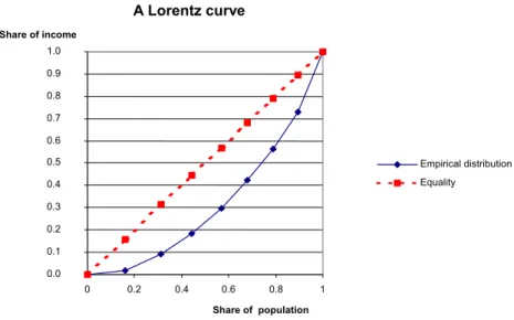
Indicators of income inequality
If everyone had the same income, every ten percent of the population would have ten percent of the income, and the straight line "Equity." B is the measure of inequality between groups, which is the result of abstracting all income differences within groups. ng/n) is the weight of the inequality within group g in the overall measure S0.
Intragenerational equity objectives and indicators
Instead of the distribution of net benefits, we might be interested in the distribution of affordability as measured by an affordability index (see, for example, Geurs and Ritsema van Eck (2001) for a review of affordability measures). The number of consumption units in the household is given by the sum of the weights of all household members.
Proposed set of indicators and targets
The same form of generalized income was also used for the same purpose in the AFFORD project (Fridstrøm et al 2000), although the Gini coefficient was used there. With regard to a target of keeping benefits within the city, the indicator will be government revenues as a percentage of the total net benefits in the strategy.
Future development
Targets could be set in terms of a mix of the indicator values for different years. The mixture that recommends itself is to use the weights on annual values used in the target function.
Vulnerable user accidents
We need livable road indicators to help us evaluate urban land use and transport strategies in relation to achieving the hard-to-quantify objectives of a vibrant, thriving and safe inner city. city and safe outdoor conditions for children in residential areas. While the former can be included in economic efficiency calculations if data are available, the latter cannot.
Double-counting
Local activity index
Proposed approach
Deriving the CO 2 cost
For the EU, the Kyoto target was then transformed into a national target for each EU country. The actual scenario we assume and the strategies we test may be with or without such a tax, but the short and long term CO2 indicator will be the same regardless.
The short term (2010) CO 2 cost
The most important choice for the tax to achieve the short-term target appears to be the assumption about international trade in permits and other implementation mechanisms. This tax can be interpreted as equal to the marginal cost to society of meeting the Kyoto CO2 target in a cost-efficient way.
Applying the CO 2 cost
There may be other equally effective ways of achieving the goal that one could assume instead. The marginal social cost of CO2 emissions will remain the same under such alternative assumptions.
The longer term (2020) CO 2 costs
The target tax rises gradually from the stabilization level of 750 to 550, but sharply from 550 to 450. Assuming that the tax gradually increases from 50 to 200 between 2010 and 2020, there should already be a significant proportion of cars on alternative fuels. .
City targets and city fuel taxes
If say 25% of the fleet emits no CO2, or all vehicles emit 25% less on average, in our calculations it is as if the tax were 150 per ton. Finally, if we want to model a case where political resistance prevents national CO2 policy, we need to reduce taxes as perceived by travelers and transport companies and the government.
What if recent fuel taxes differ from those in the CO 2 cost estimate?
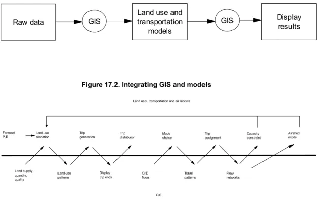
However, we do not know what level of ambition with regard to atmospheric CO2 such a target would represent. The new possibilities for visualizing model results offered by GIS can be fully exploited only if simple rules for effective visual communication are followed.
Visualisation using maps
Central to maintaining clarity in the face of the complex are graphic methods that organize and order the flow of graphic information presented to the eye (Tufte 1984). A particularly effective device for enhancing the explanatory power of a map is to add the time dimension to the design of the graphic.
Basics and potential of GIS (Geographic Information System)
Linear features, such as roads and rivers, can be stored as a collection of point coordinates. Polygonal features, such as area boundaries and school districts, can be stored as a closed coordinate circle.
Other Presentation Methods
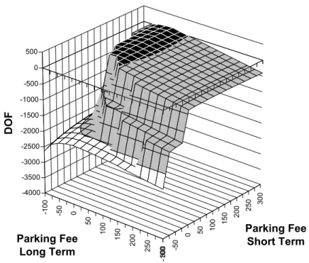
Objective function variation for the objective function DOF with variation in long- and short-term parking changes. Sensitivity test of operating costs for public transport frequency increase in the target function HOF.
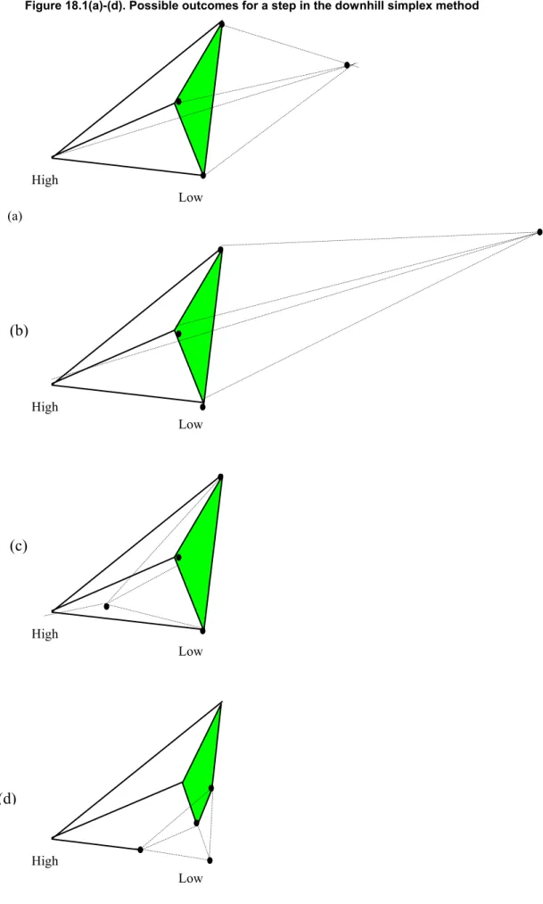
The downhill simplex method (AMOEBA)
The simplex at the end of the step (drawn with dotted line) can be:. a) a reflection away from the highest point,. In the centralized approach, all policies are optimized simultaneously to find the minimum of the target function.
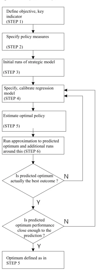
The regression approach to optimisation
The process has not converged if35. i) the regression value is more than 10% greater than the true value of the transport model run;. When trying to maximize the dependent variable, we want the fit (i.e., the quadratic approximation) to be best for the higher values of the dependent variable.
Constrained optimisation of the OF function
At the most general level, we provide a logical structure to the planning process (Section 2.2) and discuss its implication for each of the steps in the process. This type of advice is contained in the Decision Makers Guide and in Chapters 1-2 of the current guide.
PROSPECTS experience
For Vienna, the optimal strategy found in the initial optimization of the common instrument set suggests halving peak and off-peak public transport fares in 2006 as well as in 2016. The fuel tax should increase by about 20% in 2006. and fell back to the same level as in the starting year in 2016.
Experience with individual indicators and parameters